Mathovia

Calculus / Calculus 1 · Integrals

Riemann Sums

A Riemann sum estimates the area under a curve by splitting it into thin rectangles and adding up their areas. Left, right and midpoint sums differ only in where each rectangle's height is measured, and as the rectangles get thinner, the sum approaches the exact area.

Practice Problems
Written by
MPhil in Mathematics, Founder of Mathovia
Published

Mathematics verification: Mathematical formulas, calculations, worked examples and solutions are reviewed for accuracy before publication. How we check our work

A Riemann sum estimates the area under a curve by adding up the areas of thin rectangles:

Each rectangle has width and height , the value of the function at a point in its piece of the interval. Using the left endpoints, the right endpoints or the midpoints gives the left, right and midpoint Riemann sums. With more and thinner rectangles the estimate gets better, and in the limit it gives the exact area. That limit is the definite integral, the second big idea of calculus after the derivative.
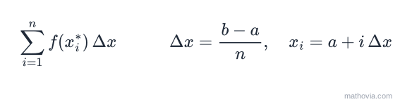
The Riemann sum: the sum from i equals 1 to n of f of x i star times delta x, where delta x equals b minus a over n and x i equals a plus i delta x
The Riemann sum formula with n equal subintervals

The Area Under a Curve

How do you find the area under the curve between and ? The region has a curved top, so no geometry formula fits it. But rectangles are easy: their area is width times height.

The idea is to cut the region into thin vertical strips and replace each strip by a rectangle. The rectangles don’t fit the curve exactly, so their total area is an estimate. Thinner strips leave less room for error, and the estimate improves.

For this region, the exact area turns out to be . Every sum in this lesson estimates that number, so you can see how close each method gets.

The Riemann Sum Formula

To build a Riemann sum for on with rectangles of equal width:

  1. Width. Each subinterval has width

  1. Endpoints. The subintervals start at and step by :

So the th subinterval is , and .

  1. Sample points. Pick a point in each subinterval. The rectangle on that subinterval has height .

  2. Add. The Riemann sum is

The is sigma notation: it means “add up the terms for to .” Because every rectangle has the same width, you can add the heights first and multiply by once at the end.

The three standard choices of sample point give three formulas:

SumSample point Formula
Left ()left endpoint
Right ()right endpoint
Midpoint ()midpoint

The next three sections work out each sum for the same region: on with . Then , and the endpoints are 0, 0.5, 1, 1.5 and 2.
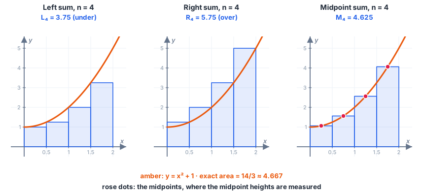
Three graphs of y equals x squared plus 1 on the interval from 0 to 2, each with four rectangles of width 0.5. Left: heights from the left endpoints, the rectangles sit below the curve, total 3.75. Right: heights from the right endpoints, the rectangles stick out above the curve, total 5.75. Midpoint: heights from the midpoints, the rectangles cross the curve, total 4.625. The exact area is 14 over 3, about 4.667
Left, right and midpoint Riemann sums for x² + 1 on [0, 2] with n = 4

Left Riemann Sum

A left Riemann sum uses the left endpoint of each subinterval for the height:

It uses every endpoint except the last one, .

Example 1. Find for on .

The left endpoints are 0, 0.5, 1 and 1.5:

00.511.5
11.2523.25

That’s below the exact area of 4.667. The function is increasing, so each rectangle’s height comes from the lowest point of its strip, and every rectangle sits under the curve.

Right Riemann Sum

A right Riemann sum uses the right endpoint of each subinterval:

It uses every endpoint except the first one, .

Example 2. Find for on .

The right endpoints are 0.5, 1, 1.5 and 2, with -values 1.25, 2, 3.25 and 5:

This time the estimate is too big. For an increasing function, each height comes from the highest point of its strip, so every rectangle sticks out above the curve.

Notice that and share the middle values 1.25, 2 and 3.25. They differ only in the ends: . Here that’s .

Midpoint Riemann Sum

A midpoint Riemann sum measures each height at the middle of its subinterval:

The midpoints are not endpoints, so list them first. Each one is halfway between two neighbouring endpoints, or equivalently .

Example 3. Find for on .

The midpoints of , , and are 0.25, 0.75, 1.25 and 1.75:

0.250.751.251.75
1.06251.56252.56254.0625

That’s within 0.042 of the exact area, much closer than the left or right sum with the same four rectangles. Each midpoint rectangle overshoots the curve on one side of its strip and undershoots on the other, and the two errors nearly cancel.

Overestimate or Underestimate?

You can often tell whether a sum is too big or too small without knowing the exact area.

Left and right sums depend on whether is increasing or decreasing:

Left sumRight sum
increasingunderestimateoverestimate
decreasingoverestimateunderestimate

Midpoint (and trapezoidal) sums depend on concavity:

Midpoint sumTrapezoidal sum
concave upunderestimateoverestimate
concave downoverestimateunderestimate

For , which is increasing and concave up on , that predicts and . The numbers agree: .

If changes direction or concavity inside the interval, these rules don’t apply to the whole sum. Check each piece separately, or just compare with the exact value.

The Trapezoidal Sum

Replace each rectangle with a trapezoid that joins the two points on the curve. That gives the trapezoidal sum, which is simply the average of the left and right sums:

For our example, . It isn’t a Riemann sum in the strict sense, since its pieces aren’t rectangles, but AP Calculus asks for it alongside the other three. Numerical methods such as the trapezoidal rule and Simpson’s rule build on this idea in Calculus 2.

Riemann Sums From a Table

In applied problems you often have a table of measurements instead of a formula. The method is the same, but the subintervals can have different widths, so multiply each height by its own width.

Example 4. Water flows into a tank at rate , in liters per minute. Estimate the total water that flows in from to with a left and a right Riemann sum.

(min)0259
(L/min)471012

The subintervals are , and , with widths 2, 3 and 4.

Left sum: use the left value of each subinterval.

Right sum: use the right value of each subinterval.

Rate times time is an amount, so the area under a rate graph is a total. That’s why Riemann sums answer “how much in total” questions, from liters of water to miles driven.

Example 5 (midpoint sum from a table). Estimate the distance traveled from to seconds with a midpoint sum and two subintervals.

(s)02468
(m/s)13689

Two subintervals means and , each 4 seconds wide. Their midpoints are and , and the table gives and :

A midpoint sum from a table only works when the table includes the midpoints. That’s why such questions use fewer, wider subintervals than the table has.

More Rectangles: The Limit of a Riemann Sum

Here are the sums for on as the number of rectangles grows:

43.75005.75004.6250
84.18755.18754.6563
164.42194.92194.6641
324.54304.79304.6660
1004.62684.70684.6666
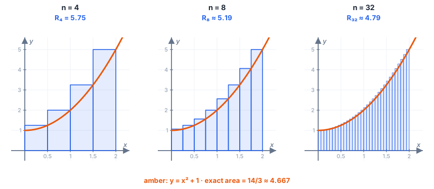
Three graphs of y equals x squared plus 1 on 0 to 2 with right Riemann sums of 4, 8 and 32 rectangles. The gaps between the rectangles and the curve shrink as the rectangles get thinner, and the sums 5.75, 5.19 and 4.79 approach the exact area 4.667
Thinner rectangles leave less error: right sums with n = 4, 8 and 32

All three columns head toward . The exact area is defined as this limit:

For a continuous function, the limit is the same whichever sample points you use. When it exists, it’s called the definite integral of from to , written . That’s the subject of the next lesson.

Example 6. Find the exact area under on as a limit of right Riemann sums.

Here and , so :

The sum of the first squares is (see the summation formulas), so

As , the top and bottom both grow like . By the rule for limits at infinity, the limit is the ratio of leading coefficients:

The exact area is 9. This works, but it’s slow, and it needs a summation formula for every new function. The fundamental theorem of calculus will get the same answer in one line from an antiderivative.

Negative Values and Net Area

If on part of the interval, the “height” is negative there, and so is the rectangle’s contribution. A Riemann sum then measures net (signed) area: area above the x-axis counts as positive, area below counts as negative.

Example 7. Find for on .

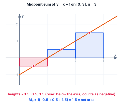
, and the midpoints are 0.5, 1.5 and 2.5:

The line y equals x minus 1 on 0 to 3 with three midpoint rectangles of width 1. The first rectangle hangs below the x-axis with height negative 0.5 and is shaded rose as negative area. The other two sit above the axis with heights 0.5 and 1.5. The net sum is 1.5
Rectangles below the x-axis count as negative area

The triangle below the axis has area 0.5 and the one above has area 2, so the net area is . The midpoint sum is exact here because is a straight line. If you want the total area instead, with every region counted as positive, add the regions’ areas separately: .

Common Mistakes

  • Using heights. A sum with rectangles uses heights. The left sum skips ; the right sum skips .
  • Using endpoints for a midpoint sum. List the midpoints first, then evaluate there.
  • Forgetting . Adding the heights isn’t enough; multiply by the width.
  • Assuming equal widths in a table. Check the gaps between the -values and multiply each height by its own width.
  • Judging the midpoint sum by increasing/decreasing. Over or under for the midpoint and trapezoidal sums depends on concavity.
  • Dropping the sign below the axis. Negative function values give negative rectangle areas, so a Riemann sum gives net area.

For more worked examples with sigma notation, see Section 5.1 of the free textbook OpenStax Calculus Volume 1.

Practice Problems

Try each one before opening the answer. The practice set has 12 more with instant checking.

Problem 1. Find for on .

Show answer

, and the left endpoints are 0, 1, 2 and 3: .

Answer:

Problem 2. Find for the same function and interval.

Show answer

The right endpoints are 1, 2, 3 and 4: .

Answer:

Problem 3. Find for the same function and interval.

Show answer

The midpoints are 0.5, 1.5, 2.5 and 3.5: . The exact area is , so the midpoint sum is a slight underestimate, as expected for a concave-up function.

Answer:

Problem 4. Find for on .

Show answer

, and the right endpoints are 2, 3 and 4: .

Answer:

Problem 5. Use the table and a right Riemann sum to estimate the distance traveled from to .

(h)0136
(km/h)40505560
Show answer

The widths are 1, 2 and 3: .

Answer: 340 km

Problem 6. is decreasing and concave up on . Is the right Riemann sum an overestimate or an underestimate? What about the midpoint sum?

Show answer

Decreasing means each right endpoint is the lowest point of its strip, so the right sum is an underestimate. Concave up means the midpoint sum is also an underestimate.

Answer: both are underestimates

Riemann sums turn area into a limit of sums. Next, the definite integral gives that limit a name and a notation, and the fundamental theorem of calculus then connects it back to antiderivatives.

Frequently Asked Questions

What is a Riemann sum?+

A Riemann sum is an estimate of the area under a curve on an interval . You cut the interval into pieces, build a rectangle on each piece whose height is a value of , and add the rectangle areas: . As grows, the estimate approaches the exact area, which is the definite integral.

What is the formula for a Riemann sum?+

With equal subintervals, the width is and the endpoints are . A Riemann sum is , where is a sample point in the th subinterval: the left endpoint , the right endpoint , or the midpoint .

How do you do a midpoint Riemann sum?+

Find , list the midpoints of the subintervals (halfway between consecutive endpoints), evaluate at each midpoint, add the values and multiply by . For on with , the midpoints are 0.25, 0.75, 1.25 and 1.75, and the sum is .

Is a midpoint Riemann sum an overestimate or an underestimate?+

It depends on concavity, not on whether the function rises or falls. If is concave up, the midpoint sum is an underestimate; if is concave down, it is an overestimate. For a straight line it is exact. Left and right sums depend on monotonicity instead: for an increasing function the left sum is under and the right sum is over.

What is the difference between left and right Riemann sums?+

Both use the same subintervals. A left Riemann sum takes each rectangle's height from the left endpoint, so it uses through . A right Riemann sum uses the right endpoints, through . The two sums share every middle term and differ only in the first and last ones.

How is a Riemann sum related to the definite integral?+

The definite integral is the limit of Riemann sums as the number of rectangles goes to infinity: . For a continuous function the limit is the same whichever sample points you use, so left, right and midpoint sums all approach the same number.

Related lessons