Mathovia

Calculus / Calculus 1 · Applications of Derivatives

Linear Approximation

Linear approximation replaces a curve with its tangent line near a point you know well. The tangent line is easy to evaluate, and close to that point it gives almost the same values as the function.

Practice Problems
Written by
MPhil in Mathematics, Founder of Mathovia
Published

Mathematics verification: Mathematical formulas, calculations, worked examples and solutions are reviewed for accuracy before publication. How we check our work

Chapter 4 · Lesson 2 of 5Calculus 1 · Applications of Derivatives
  1. 1.Related Rates
  2. 2.Linear Approximation
  3. 3.Critical Points
  4. 4.Extreme Value Theorem
  5. 5.Rolle's Theorem
See all calculus chapters →

What is ? You can’t get it exactly by hand, but you know , and 26 is very close to 25. Linear approximation uses that: near a point you know, a smooth curve is almost the same as its tangent line, and a line is easy to evaluate. The same idea is behind the small-angle approximation in physics, Newton’s method for solving equations, and estimating how measurement errors spread through a calculation.

The linearization L of x equals f of a plus f prime of a times x minus a, and f of x is approximately L of x for x near a
The linearization is the tangent line at x = a

What Is Linear Approximation?

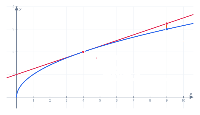
The curve y equals square root of x and its tangent line L of x equals 2 plus one quarter of x minus 4, touching at 4, 2. Near x equals 4 the two are almost equal. At x equals 9 the tangent line gives 3.25 while the square root of 9 is 3, an error of 0.25
The tangent line hugs √x near x = 4 and drifts away farther out

The linearization of at is the tangent line at that point, written as a function:

Linear approximation means using in place of for values of close to :

The graph shows why this works. At the line and the curve meet and have the same slope, so they leave that point heading in the same direction. Close to they’re nearly indistinguishable. Farther away the curve bends and the line doesn’t, so the error grows. The approximation is a local one: it’s only good near .

The point is called the center of the linearization. Choose it close to the value you want, at a place where and are easy to compute exactly.

How to Do a Linear Approximation

  1. Choose : a nearby value where the function is easy to evaluate.
  2. Compute and .
  3. Write .
  4. Evaluate at the value you want.

Example 1: Estimating a Square Root

Estimate .

Step 1 — choose : and , since exactly.

Step 2 — the value and slope at :

Step 3 — the linearization:

Step 4 — evaluate:

The true value is , so the estimate is off by less than 0.001.

Example 2: A Cube Root

Estimate .

Use at . Then and , so :

The true value is .

Example 3: Approximations Near Zero

Many standard approximations come from linearizing at . For , and , so :

That’s the small-angle approximation from physics: , and the true value is . The same steps give the whole table:

FunctionLinearization at ExampleEstimateTrue value

The last row is worth remembering. is why 1% growth for 10 years is roughly, but a bit more than, 10% in total.

Overestimate or Underestimate?

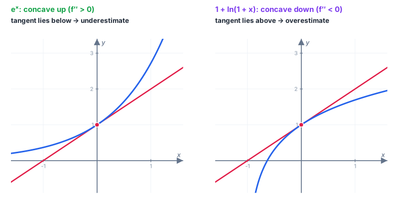
Two graphs. Left: e to the x is concave up and its tangent line at 0, 1 lies below the curve, so the linear approximation underestimates. Right: 1 plus ln of 1 plus x is concave down and its tangent line at 0, 1 lies above the curve, so the linear approximation overestimates
Concave up: the tangent line is below the curve. Concave down: above

The second derivative tells you which side of the curve the tangent line is on:

  • , concave up: the curve bends up away from the tangent line, so the line is below the curve and is an underestimate.
  • , concave down: the line is above the curve and is an overestimate.

Check this against the examples. For , , so 5.1 should be too big, and it is: . For , , so 1.05 should be too small, and it is: .

How Accurate Is It?

The error depends on two things: how far is from , and how sharply the curve bends. Back to at , where :

Error
4.12.0252.024850.00015
52.252.236070.014
93.2530.25

Moving 10 times farther from (from 0.1 to 1) makes the error about 100 times bigger. That’s typical: the error grows roughly with the square of the distance from . Taylor polynomials, later in the course, fix this by adding a curved correction.

Differentials

The same idea, written in terms of changes, is called differentials. Let be a small change in . The matching change along the tangent line is
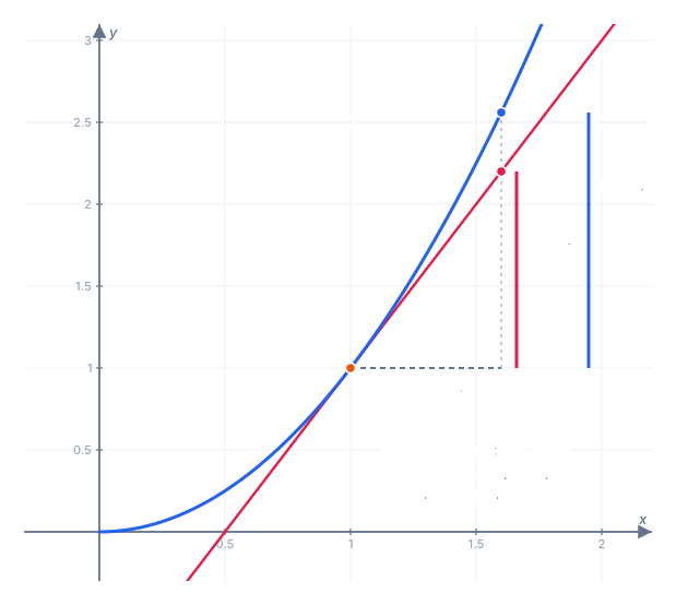
The curve y equals x squared with its tangent line at 1, 1. Moving right by dx equals 0.6, the tangent line rises dy equals 1.2 while the curve rises delta y equals 1.56
dy is the rise along the tangent line; Δy is the rise along the curve

The true change in the function is , and for small , . On at with , while . That’s a large , chosen so the gap is visible. With , and .

Estimating Measurement Error

Differentials are how scientists estimate how an error in a measurement affects a result. Suppose a ball’s radius is measured as 10 cm, with a possible error of 0.1 cm. How far off could the computed volume be?

Step 1 — the volume and its differential:

Step 2 — substitute , :

Step 3 — compare to the volume. cm³, so the relative error is

A 1% error in the radius becomes about a 3% error in the volume. The exponent 3 in triples the relative error.

Common Mistakes

  • Choosing far from . The approximation is only accurate near . For , works; gives 5.25, which is much worse.
  • Using degrees in trig approximations. only holds in radians. is about 0.087, not 5.
  • Evaluating at instead of . The slope in is the number .
  • Mixing up and . is the tangent-line estimate; is the exact change. They’re close only when is small.

Practice Problems

Try each one before opening the answer. The practice set has 12 more with instant checking.

Problem 1. Find the linearization of at .

Show answer

Step 1 — the value and slope:

Step 2 — the linearization:

Answer:

Problem 2. Use a linear approximation to estimate .

Show answer

Use : and .

Answer: (true value )

Problem 3. Estimate .

Show answer

Use at : and .

Answer: (true value )

Problem 4. Use the linearization of at to estimate .

Show answer

and , so .

Answer: (true value )

Problem 5. Is the estimate from Problem 2 too high or too low?

Show answer

, which is negative, so is concave down and its tangent line lies above it.

Answer: too high, an overestimate

Problem 6. The side of a square is measured as 5 cm, with a possible error of 0.02 cm. Use differentials to estimate the possible error in its area.

Show answer

Answer: about cm²

The tangent line has now given you slopes, equations and estimates. Next, the derivative helps find where a function reaches its highest and lowest values, starting with critical points.

Frequently Asked Questions

What is linear approximation?+

Linear approximation estimates the value of a function near a point by using the tangent line at instead of the function itself. Close to , the curve and its tangent line are almost the same, so .

What is the linear approximation formula?+

The formula is . Here is a point where you know and exactly, and approximates for near .

What is the difference between linear approximation and linearization?+

They describe the same idea. The linearization is the function itself, and linear approximation is the act of using to estimate .

How do you choose the point a?+

Pick a value close to the number you want where and are easy to compute exactly. To estimate , use , because is exact and 25 is close to 26.

How do you know if a linear approximation is an overestimate or an underestimate?+

Look at the second derivative. If , the curve is concave up, the tangent line lies below it, and the approximation is an underestimate. If , the curve is concave down and the approximation is an overestimate.

What are differentials?+

Differentials are the change along the tangent line: . For a small change in , approximates the true change in the function. They're used to estimate how much a measurement error in affects a computed quantity.

Related lessons