Binomial Distribution Calculator

A binomial distribution answers a question people ask all the time without naming it: if something has a fixed chance of happening on every try, how likely is it to happen a certain number of times? Guessing on a multiple-choice quiz, free throws in a game, defective parts in a box of twelve. Each one is a count of successes across repeated, independent tries, and the binomial formula gives you the exact odds of every possible count.

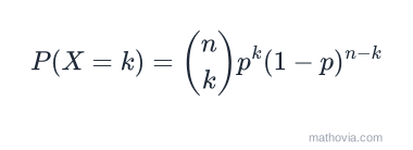
The binomial probability formula

The probability of getting exactly successes in trials is

Each piece has a job. is the chance that k particular trials all succeed. is the chance that the remaining trials all fail. And the binomial coefficient , read “n choose k”, counts how many different ways those k successes can be scattered across the n trials, because getting the right answers on questions 1, 2 and 3 is a different outcome from getting them on questions 4, 7 and 9, yet both count as “3 correct”.

Before you trust any binomial answer, check that the situation actually fits. You need a fixed number of trials, two outcomes per trial (success or failure), the same on every trial, and trials that don’t influence each other. A quiz where every question has four options passes. Drawing five cards from a deck without putting them back doesn’t, since the odds shift after every draw.

How to calculate a binomial probability (step by step)

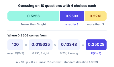
The calculator’s defaults describe a familiar situation: you guess blindly on a 10-question quiz where each question has 4 options. So n = 10, p = 0.25, and we want the probability of getting exactly x = 3 right.

Step One: Count the arrangements with n choose k

C(n, k) = n! / (k! × (n − k)!)

C(10, 3) = 10! / (3! × 7!) = (10 × 9 × 8) / (3 × 2 × 1) = 720 / 6 = 120

There are 120 different ways to pick which 3 of the 10 questions you get right.

Step Two: Find the probability of one specific arrangement

p^k × (1 − p)^(n − k)

0.25^3 = 0.015625
0.75^7 = 0.13348
0.015625 × 0.13348 = 0.0020857

That tiny number is the chance of one particular pattern, say right on questions 1 to 3 and wrong on the other seven.

Step Three: Multiply to get P(X = x)

P(X = 3) = 120 × 0.0020857 = 0.25028

So a pure guesser hits exactly 3 out of 10 about 25% of the time. That matches the calculator’s primary result, P(X = x) = 0.25028.

Step Four: Add terms for the cumulative probabilities

A cumulative probability is just a sum of exact probabilities. “At most 3” means 0, 1, 2 or 3 correct:

P(X ≤ 3) = P(0) + P(1) + P(2) + P(3)
         = 0.056314 + 0.187712 + 0.281568 + 0.250282 = 0.77588

The other tails come from the same pieces:

P(X < 3) = P(0) + P(1) + P(2)  = 0.525594 → 0.52559
P(X > 3) = 1 − P(X ≤ 3)        = 1 − 0.77588 = 0.22412
P(X ≥ 3) = 1 − P(X < 3)        = 1 − 0.52559 = 0.47441

Keep at least six decimals in the individual terms when you add by hand. Rounding each one to five places first can push the last digit of the total off by one.

Step Five: Find the mean, variance and standard deviation

mean     μ  = n × p           = 10 × 0.25         = 2.5
variance σ² = n × p × (1 − p) = 10 × 0.25 × 0.75  = 1.875
std dev  σ  = √1.875                              = 1.3693

On average a guesser gets 2.5 questions right, and most results land within about 1.4 of that.

Reading the full distribution

Here is every outcome for the guessing example. The cumulative column is P(X ≤ k), the number a TI-84’s binomcdf would give you.

Two things stand out. The most likely single result is 2, not the mean of 2.5, because the count has to be a whole number. And passing by luck is close to hopeless: scoring 6 or more (a 60%) has a probability of about 0.0197, roughly one guesser in fifty. If you’d rather think in percentages, multiply by 100, or run any value through the fraction to percent calculator.

Which probability should you use?

Most homework mistakes come from picking the wrong tail, not from bad arithmetic. Translate the wording first:

• “exactly 3”: P(X = 3)
• “at most 3”, “no more than 3”, “3 or fewer”: P(X ≤ 3)
• “fewer than 3”, “less than 3”: P(X < 3), which is P(X ≤ 2)
• “at least 3”, “3 or more”, “no fewer than 3”: P(X ≥ 3)
• “more than 3”, “over 3”: P(X > 3), which is P(X ≥ 4)

“At least one” problems deserve a special mention, because the complement makes them easy. A factory part fails 5% of the time and you install 12 of them. The chance that none fail is 0.95¹², about 0.5404, so the chance that at least one fails is about 0.4596. Set n = 12, p = 0.05 and x = 0 and the calculator shows that as P(X > 0). Nearly a coin flip, even with a part that’s 95% reliable. That surprises people every time.

Real situations where the binomial shows up

A basketball player who makes 90% of free throws takes 20 of them. The chance she makes exactly 17 is 0.1901, and the chance she makes at least 17 is 0.8670. Her chance of a perfect 20 for 20? Only 0.1216, which is why perfect nights are rarer than shooting percentages suggest.

Quality control runs on the same math. If 2% of light bulbs are defective, an inspector who samples 50 bulbs from a perfectly normal batch will still find 2 or more bad ones about 26% of the time (P(X ≥ 2) = 0.2642). A rule of “reject at 2 defects” would throw out one good batch in four, so the cutoff has to sit higher than intuition suggests. Clinical trials, A/B tests and polling all lean on the same idea. Count the yes answers and ask whether that count is plausible under a given p.

Common mistakes

1. Using a percentage for p. Enter 0.25, not 25. The probability has to sit between 0 and 1.
2. Forgetting the n choose k factor. on its own is the chance of one specific order, and it’s usually far too small.
3. Off-by-one tails. “More than 3” starts at 4. Write the inequality down before you calculate.
4. Applying it to dependent trials. Without replacement, the probability changes from draw to draw, and the binomial overstates the spread.
5. Rounding p before multiplying. Keep full precision through the calculation and round only the final answer. The powers magnify small rounding errors.

The exponent steps are ordinary power rules, and the exponent rules lesson is a quick refresher if looks intimidating. For more practice turning probabilities into percents and back, try the percentage problem generator.